In previous posts, we provided examples of pricing European and American options in Excel. For pricing the European option, we utilized the Black-Scholes formula, and for pricing the American option we utilized the binomial approach. In this post, we are going to implement these methods in Python.
Recall that,
In finance, the binomial options pricing model (BOPM) provides a generalizable numerical method for the valuation of options. The binomial model was first proposed by Cox, Ross and Rubinstein in 1979. Essentially, the model uses a “discrete-time” (lattice based) model of the varying price over time of the underlying financial instrument…
The binomial pricing model traces the evolution of the option’s key underlying variables in discrete-time. This is done by means of a binomial lattice (tree), for a number of time steps between the valuation and expiration dates. Each node in the lattice represents a possible price of the underlying at a given point in time.
Valuation is performed iteratively, starting at each of the final nodes (those that may be reached at the time of expiration), and then working backwards through the tree towards the first node (valuation date). The value computed at each stage is the value of the option at that point in time. Read more
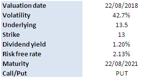
We use the same input parameters as in the previous examples. The main input parameters are as follows,

Figure below shows the results calculated by the Python program. The Python program returns the same values as the Excel workbooks.
![]()
To download the accompanying Excel workbook or Python program for this post:
1. Subscribe to the newsletter. If you're already a subscriber, go to the next step
2. Once subscribed, refer a friend
After completing these steps, you’ll gain access to the file for this post, along with files for a dozen other posts.
Further questions
What's your question? Ask it in the discussion forum
Have an answer to the questions below? Post it here or in the forum


Thank you.